Marginal Cost, Average Variable Cost and Average Fixed Cost (transcript)

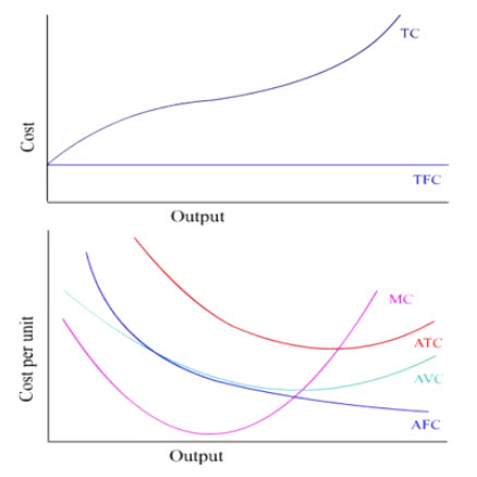
Marginal cost, average variable cost and average fixed cost can be derived from a short-run production function subject to the law of diminishing returns.

Generating MC from TVC

In the short run where some fixed inputs are combined with variable inputs, the production function is an S-shaped upward sloping curve (TP). This total product curve starts with a segment with increasing slope followed by a segment with decreasing slope reflecting the law of diminishing returns.

From this TP curve, we can derive the total variable cost curve.

In the TP curve, output is a function of variable input. By reversing the horizontal and vertical axis, we get TVI (total variable input).

The new (flipped) curve shows variable input as a function of output.

If we multiply TVI by a constant unit cost of the variable input, we get TVC (total variable cost). Here we assume the constant unit cost is $1, so the vertical axis retains the same scale and is simply relabeled as cost.

The rate at which TVC increases is gauged by the slope of the tangent to TVC at a given output level.

At Q1, for example, the slope of the tangent to TVC simply indicates the amount of additional variable cost required to produce one more unit of output at Q1.

The numerical value of this slope is called marginal cost (MC) and is plotted on the graph below.

Given the inverted S-shape of TVC, MC first decreases...

until MC reaches its minimum at the inflection point.

Then, MC increases after the inflection point.

Thus, the inverted S-shaped TVC generates a U-shaped MC

The U shape of MC is a reflection of first increasing returns followed by decreasing returns as more and more variable input is combined with the short-run fixed input.

From TVC to AVC

When TVC is divided by a given level of total output, we get average variable cost (AVC).

At Q1, AVC = TVC1/Q1.

Since TVC1/Q1 also measures the slope of the ray from the origin to TVC, the ray slope provides a visual indication of the numerical value of AVC.

Whereas MC is the slope of the tangent at that point.

MC1 is below AVC1 because the slope of the tangent (MC1) is flatter than the ray slope from the origin (AVC1).

Given the inverted S-shape of TVC, AVC first decreases...

until it reaches the point on TVC where the ray from the origin is tangent to TVC.

Afterwards, the slope of rays from the origin to TVC starts to increase...

giving AVC a U-shape.

Observations

First, AVC reaches its minimum when the ray from the origin is tangent to TVC.

Since the slope of this tangency measures both MC and AVC, MC therefore intersects AVC at AVC's minimum point.

Second, AVC has a symmetric U-shape because two points on opposite sides of the minimum AVC point on TVC have equal slopes.

Third, When AVC is decreasing, MC is always below AVC.

Fourth, When AVC is increasing, MC is always above AVC.

Generating AFC from TFC

When the cost of fixed inputs is added, TVC is simply shifted up by the same amount over the whole range of output.

When TFC is divided by a given level of total output, we get AFC (average fixed cost)

At Q1, AFC = TFC1/Q1.

Since TFC1/Q1 also measures the slope of the ray from the origin to TFC, the ray slope provides a visual indication of the numerical value of AFC.

Because TFC is a horizontal straight line, the slope of rays from the origin will uniformly decrease as output increases.

AFC is therefore a decreasing curve.

From AFC and AVC to ATC

With the average variable cost, AVC (animate and pause) and average fixed cost, AFC (animate and pause), we can construct the average total cost, ATC.

Since ATC = AVC + AFC, we can add AFC to AVC graphically.

For example, ATC1 = AFC1 + AVC1

Similarly, we can derive other ATC points and finally the ATC curve.

Alternatively, we can derive the ATC curve by measuring the slope of the rays from the origin to TC.

Here is the side-by-side comparison.

These two methods generate identical ATC's.

Notice that the gap between ATC and AVC is narrowing with higher output because AFC is falling as output increases.

And MC always intersects ATC and AVC at their minimum points.

Why AVC and ATC?

Why do we need AVC as well as ATC?

In the short run, the fixed inputs must be paid for whatever the level of output might be. So as long as the unit price of the output is higher than AVC, some of the fixed costs will be covered. The business is better off operating than shutting down. In the long run, unit price of the output must be at least equal to ATC to cover all economic costs.

Why MC?

Why do we need MC?

We need MC because pricing should be based on MC not on ATC. To maximize profit, we need to know that unit price is not only higher than ATC (thus covering all costs), but also that the additional cost of the marginal unit of output (MC) is not higher than the unit price.